

As humans are on a continuous quest of finding their purpose in life, AI engines are exploring the optimal way to find resolutions. This is the life cycle of an AI algorithm and it has a name: searching.
Searching is a key concept in problem-solving theory. As living beings, we spend our lives solving problems continuously. In order to create an engine that imitates our behaviour, we need first to understand the definition of a problem and what are the actions that beings follow to approach and solve it. So this engine will become a problem-solving agent and its quest will be to fulfil its purpose – solving the problem it was created for, so reaching its goal.
In this article, we are discussing what problem-solving agents really are, what searching is, the different search terminologies and the different search algorithms.
So what are problem-solving agents?
In one of the previous articles, we discussed intelligent agents. In general, intelligent agents are likely to maximize their performance measures, and achieving this is sometimes simplified if the agent adopts the object and aims at satisfying it. [1] The problem-solving agent performs precisely by defining problems and their several solutions. Problem-solving refers to a state where agents wish to reach a concrete goal from a present circumstance or condition. It is a part of artificial intelligence that encompasses a number of techniques, such as algorithms and heuristics to solve a problem. [2]
A problem-solving agent is basically a goal-based agent and focuses on satisfying the goal. [2] Goals help to coordinate behaviour by defining the purposes that the agent is trying to achieve and so the steps it needs to take.
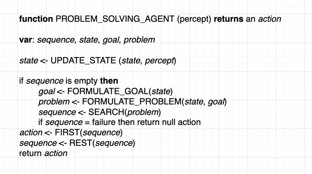
A problem-solving agent consists of goal formulation, problem formulation, search solution and execution.
- Goal formulation is based on the agents’ performance measures and the current situation of the agent. It is the simplest and the first step in problem-solving that organizes the actions required to formulate one aim out of multiple aims as well as the actions to achieve that goal. [2]
- Problem formulation is the most important step of problem-solving that decides what actions should be taken to achieve the formulated goal. [2] The process of looking for a series of steps that reached the goal is known as search. The search algorithm takes a problem as an input and returns an explanation in the form of an action sequence. [3]
- When reaching the expected resolution, the actions it recommends can be moved out. This is called the execution phase. After formulating the problem to solve and the goal, the agent calls a search method to solve it, and then uses the solution to supervise its actions, doing whatever the solution suggests, as the first action of the sequence, and then eliminating that step from the sequence. Once the solution has been performed, the agent will formulate a new goal. While executing the solution sequence the agent ignores its percept at the time of selecting an action because it has information about them in advance. An agent that carries out its methods with his eyes closed must be quite certain of what is going on. [1]
Problem definition
In general, five constituents are involved in problem formulation or a definition, namely the initial state, actions, goal test, transaction model and path cost.
- The initial state is the starting state of the agent towards its goal. Actions are the description of the possible actions that are available to the agent to reach the goal.
- Given a particular state S were actions S returns the set of actions that can be executed in S and each of these actions is applicable in S. Transition model describes what each action does specify by a function result S(A) that returns the state which results from doing action A in state S. A term successor is used to refer to any state reachable from a given state by a single action.
- Goal test determines if the given state is a goal state or not. It may be possible that there is an explicit set of possible goal states and the test simply test whether the given state is one of them or not. Sometimes, the goal is defined by an abstract property rather than an explicitly enumerated set of states.
- Path cost is a numeric cost assigned to each path that follows the goal. The problem-solving agent selects a cost function that reflects its performance measure. For an optimal solution, the path cost should be the lowest of all the solutions. [2]
The initial state, transaction model and actions together define the state-space of the problem implicitly. The state-space of a problem is a set of all states that can be reached from the initial state, followed by any sequence of actions. [4] It forms a directed map or graph, where nodes are the states, actions are the links between the nodes and the path is a sequence of states connected by a sequence of actions.
What is a search?
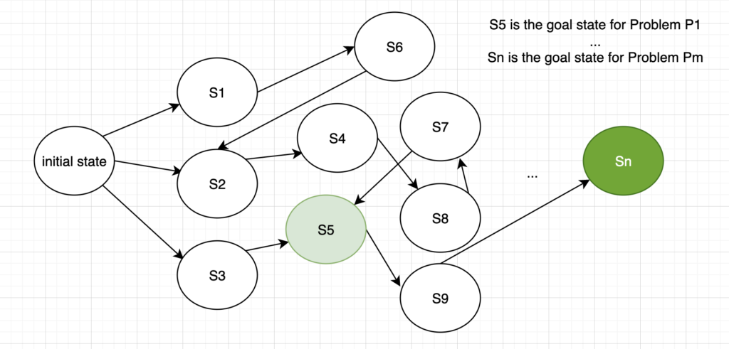
Search is the process of navigating from a starting state (initial state) to a goal state by transitioning through intermediate states. (Fig 2)
To find a solution, some sequences of actions are performed and search algorithms work by considering various possible action sequences. The possible action sequences starting at the initial state form a search tree with the initial state at the root. The branches are actions and the nodes correspond to states in the state-space of the problem. In AI, the searching techniques are strategies that look for solutions to a problem in a search space. [5]
The goal states or solutions could sometimes be an object, a goal, a sub-goal or a path to the search item.
To evaluate the algorithms’ performance, there are four ways: completeness, optimality, space complexity, and time complexity.
- Completeness refers to the algorithm guaranteed to find a solution when there is at least one solution present. [6]
- Optimality defines the strategy that is used to achieve the goal and if it finds the optimal solution or not. [7]
- Space complexity tells how much memory is needed to perform the search mechanism. [8]
- Time complexity tells how long it takes to find a solution. [8]
Time and space complexity are always considered with respect to some measure of the problem difficulty typically with the size of the state space graph. It is appropriate when the graph is in an explicit data structure that is an input to the search program.
In AI, the graph is often expressed implicitly by the initial state transition model and actions in this frequently infinite. Due to these reasons, complexity is expressed in terms of branching factors or the maximum number of successes of any node, the depth of the shallowest goal node and the maximum length of any path in the state space. [9]
Time is measured in terms of the number of nodes produced during the search in space in terms of the maximum number of nodes stored in memory.
To evaluate the effectiveness of a search algorithm, we can consider the search cost or total cost. [10] Search cost depends on the time complexity, but can also include a term for memory usage, whereas the total cost combines the search costs and the path cost of the founded solution.
Search terminologies
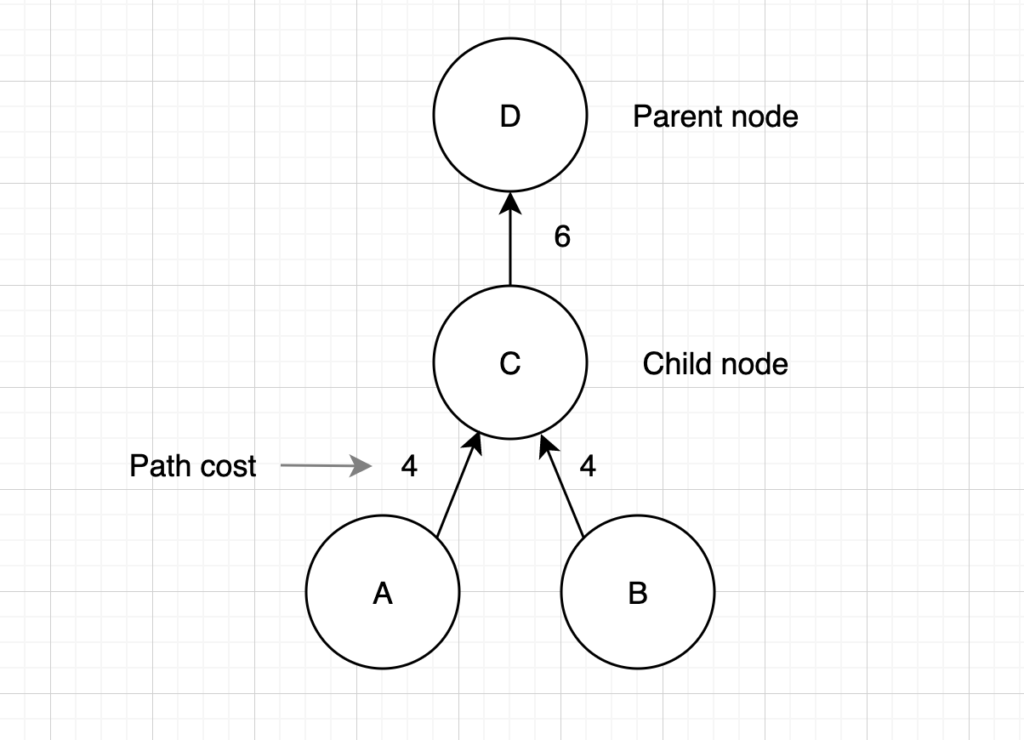
Search algorithms require a data structure to keep track of the search tree which has been constructed. For each node let’s say Node n of the tree we have a structure that contains four components: state, parent node, action and path cost. [1]
- The state is to which the node corresponds. A state can be classified as an initial state, an intermediate state or a final state. The initial state is where searching begins from, the intermediate state is the state between the starting state and the goal state that we need to transact. The goal state or final state is the state where searching stops. [11]
- Parent node, which is the node from which the current node is generated.
- An action is an operation that was applied to the parent to generate the current node.
- Path cost is the path cost from the initial state to the current node.
Transactions are the act of moving between states, in the search space that is represented by a graph – which is based on graph theory.
A branching factor is the average number of child nodes in the problem space graph. The depth of a problem is defined by the shortest path length from the initial state to the goal state. In searching, the most appropriate data structure is a queue. [12] The operations of the queue are as follows:
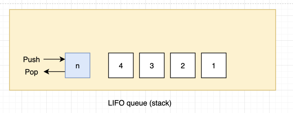
- Empty – returns true only if there are no more elements in the queue.
- Pop – removes the first element of the queue and returns it.
- Push – inserts an element and returns the result in the queue.
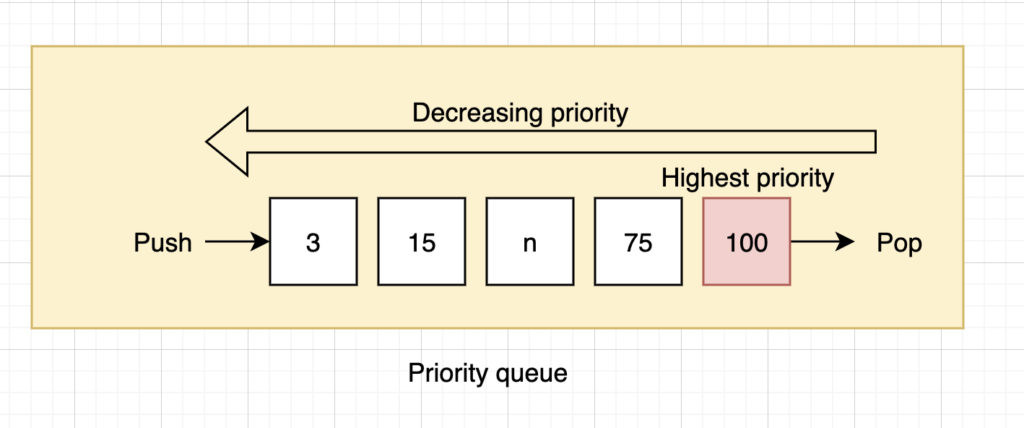
Queues are represented by the order in which they store the inserted notes. Three common queues are:
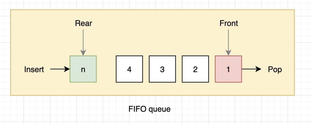
- FIFO queue or first in first out queue, which pops the oldest element of the queue
- LIFO queue that is last in first out (also known as a stack), which pops the newest element of the queue
- The priority queue – pops the element of the queue with the highest priority according to some ordering function.
Types of search algorithms in AI
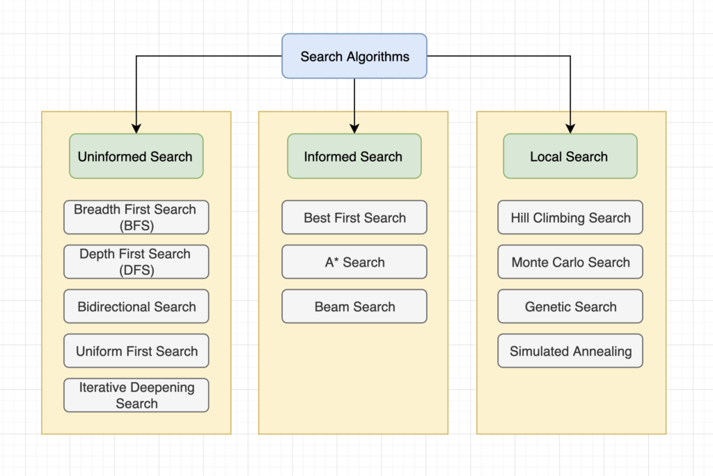
Search algorithms can be categorized as Uninformed search, Informed search and Local search.
Uninformed Search
An uninformed search is the search algorithm, which is used when there is no additional information about the goal node other than the one provided in the problem definition. [13] They simply generate successors and differentiate between the goal and non-goal states. It is also known as the blind search algorithm. The main classical uninformed search algorithms are Breadth-first search, Depth-first search, Bidirectional search, Uniform cost search and Iterative deepening search. (Fig 7)
- Depth-first search or DFS is an algorithm for searching or traversing a tree or graph data structures, starting from the root node and exploring as far as possible among each branch. [14] The search proceeds to the deepest level of the search tree. The node is expanded first, and then its successor is expanded. And this process is continued until the goal node is reached. If the latter has occurred, the search backtracks to the previous node and explores its other successor, if any of them are still unexplored. DFS is said to be a non-optimal solution and also an incomplete solution.
- Breadth-first search or BFS is an algorithm for searching for traversing tree or graph data structures initiating from the root node and exploring all the neighbour nodes at the present depth before moving on to the nodes at the next depth level. [15] It always expands the shallowest unexpanded node. And for that, it uses the first in first out (FIFO) queue for the frontier and it is said to be complete.
- Bidirectional search is a search algorithm that finds the shortest path from source to goal vertex running two simultaneous searches at a time, the forward search from the source toward the goal vertex and the backward search from goal toward the source. [16] It replaces the single search graph with two smaller subgraphs, one starting from the initial vertex and the other starting from the goal vertex. And this search terminates when two graphs intersect each other at the same point.
- Uniform cost search or UCS is used to find a path where the cumulative sum of costs is at the least. They expand the node with the least path costs first. In this, the goal tests on the node are performed when it is selected for expansion. As the first node, which is generated could be a suboptimal path. They generally provide an optimal solution because at every step, the path with the least cost is chosen and paths never get shorter as nodes are added, assuring that the search expands nodes in the order of their optimal path cost and it will get stuck in an infinite loop if there is a path with an infinite sequence of zero cost actions.
- Iterative deepening or iterative deepening depth-first search is a graph search algorithm in which depth-first search is run repeatedly with increasing debt limits until the goal is found. [17] It is optimal like breadth-first search but uses much less memory. At each iteration, it visits the nodes in the same order as the depth-first search but has the cumulative order in which nodes are first visited as breadth-first search in the tree search method.
Informed search
Informed search is the search algorithm which is used when the algorithms have information on the goal node that helps them more efficient searching. [18] This information is generally obtained by the heuristic method. Informed search can be categorized as Best first search, A* Search and Beam search. (Fig 7)
- Best first search is a graph search algorithm in which a node is selected for expansion based on the evaluation function. The node which is at the lowest evaluation is selected for the explanation because the evaluation measures the distance to the goal. The best first search algorithm can be implemented within the general search framework through a priority queue. It serves as a combination of depth-first and breadth-first search algorithms and is often referred to as the greedy algorithm because it quickly attacks the most desirable path as soon as its heuristic way becomes the most desirable.
- A* algorithm is one of the most successful search algorithms for finding the shortest path within the nodes or graphs. It is considered to be an informed search algorithm as it utilizes information about the path costs and also applies heuristics to find the solution. It is one of the most popular and best techniques used in pathfinding and graph traversals.
- Beam search is the restricted or modified version of either a breadth-first search or a best-first search algorithm. It is restricted in the same sense, but the amount of memory available for storing the set of alternative search nodes is limited. And in the sense that non-promising nodes can be pruned at any step in the search. It is a forward pruning heuristic search that takes three components as its input, which are a problem, a set of heuristic rules for pruning and the memory with a limited available capacity.
Local Search
The local search algorithm is mostly applied to problems for which information about the path to get the solution is unknown, but only information about the final solution is known. They are operated using a single state and explore the neighbours of that state and usually don’t store the path. They are generally used when there is more than one possible goal state and the best outcomes needed to discover.
The local search consists of Hill Climbing search, Monte Carlo search, Genetic search and Simulated Annealing. (Fig 7)
- Hill climbing is a greedy search method that detriments the next state based on the value that is the smallest until it hits a local maximum. [5] It is basically a mathematical optimization technique that belongs to the family of local search. Hill climbing is an iterative algorithm that starts with an arbitrary solution to a query and then tries to find a better solution by making incremental changes to the solution. If the alteration produces a better solution another incremental change is made to the solution found. It continues until no further improvements can be found.
- Monte Carlo search – Monte Carlo Tree Search for MCTS is a heuristic search algorithm for decision processes that are generally used in gameplay. [19] MCTS was introduced in 2006 and has been used in board games like chess, games with incomplete information such as poker as well as internet-based strategy video games.
- Genetic search is a metaheuristic inspired by the process of natural selection and belongs to evolutionary algorithms (EA). [20] The genetic algorithms are generally used to generate high-quality solutions for search problems and optimization by relying on bio-inspired operators, such as selection, mutation and crossover. In this algorithm, a population of candidates’ solutions to an optimization problem evolves toward better solutions. Each candidate solution has a set of treats that can be mutated and altered.
- Simulated annealing is a probabilistic method for approximating the global optimum of a given function. [21] It is a metaheuristic to approximate global optimization and a large search space for an optimization problem. It is mostly used when the search space is discrete and used for those issues, where finding an estimated global optimum is more important than finding a specific local optimum, and a fixed amount of time.
In order to prepare this article, I studied the lectures from GlobalTechCouncil. They served me as a great source of inspiration and guidance through the process of discovering and understanding AI technologies.
Below, you can also find some valuable materials on this topic.
References
[1] https://www.pearsonhighered.com/assets/samplechapter/0/1/3/6/0136042597.pdf
[2] https://www.tutorialandexample.com/problem-solving-in-artificial-intelligence
[3] https://www.massey.ac.nz/~mjjohnso/notes/59302/l03.html
[4] https://www.sciencedirect.com/topics/computer-science/state-space-problem
[5] https://towardsdatascience.com/ai-search-algorithms-every-data-scientist-should-know-ed0968a43a7a
[6] https://www-users.cse.umn.edu/~gini/4511/search
[7] https://www.sciencedirect.com/topics/engineering/optimality
[8] https://www.baeldung.com/cs/time-vs-space-complexity
[9] https://web.cs.hacettepe.edu.tr/~ilyas/Courses/VBM688/lec03_search.pdf
[10] http://web.pdx.edu/~arhodes/ai7.pdf
[11] https://socialsci.libretexts.org/Courses/Sacramento_City_College/
[12] https://www.massey.ac.nz/~mjjohnso/notes/59302/l03.html
[13] https://www.geeksforgeeks.org/difference-between-informed-and-uninformed-search-in-ai/
[14] https://www.geeksforgeeks.org/search-algorithms-in-ai/
[15] https://en.wikipedia.org/wiki/Breadth-first_search
[16] https://en.wikipedia.org/wiki/Bidirectional_search
[17] https://en.wikipedia.org/wiki/Iterative_deepening_depth-first_search
[18] https://www.javatpoint.com/ai-informed-search-algorithms
[19] https://en.wikipedia.org/wiki/Monte_Carlo_tree_search
[20] https://en.wikipedia.org/wiki/Genetic_algorithm
[21] https://en.wikipedia.org/wiki/Simulated_annealing


